Wolfram Mathematica 14.3.0 — Mac version

If you've ever stretched a spreadsheet to its limits, you'll recognise the feeling of outgrowing your tools. Mathematica picks up where that ends — symbolic algebra, differential equations, visual models. It's a desktop technical computing app from Wolfram that combines symbolic, numerical, and visual work in one place, backed by thousands of Wolfram Language functions.

Getting started: what you need and what you get

1. Check your macOS version. You need macOS 12 or later. It runs on both Intel and Apple Silicon Macs.
2. Open the notebook interface. This is where you type calculations and see results — now with full dark mode support and new standard colours for light and dark environments.
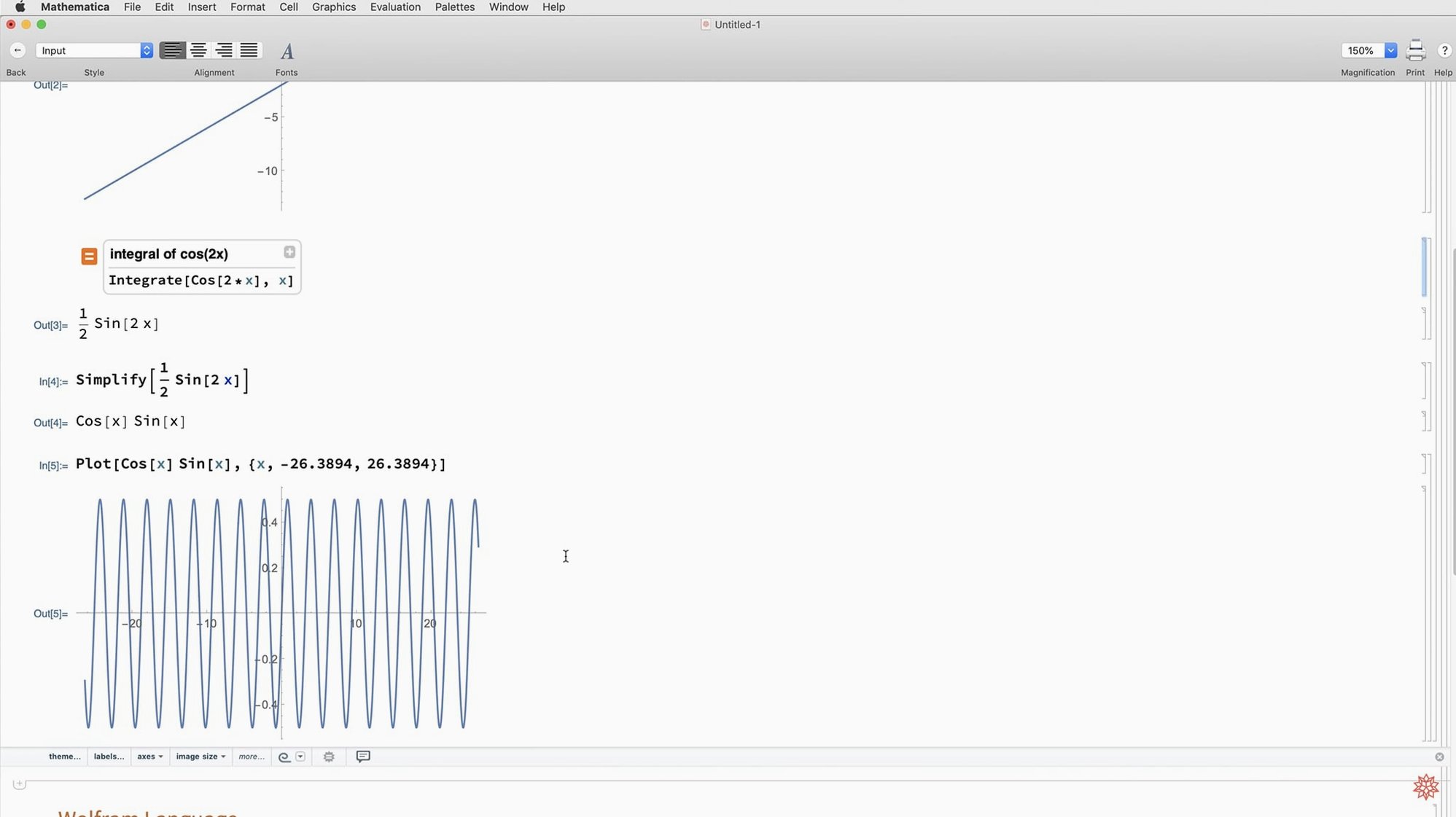
3. Try a symbolic or numerical task. Solve an equation, integrate a function, or run a matrix decomposition. Version 14.3 adds Hilbert transforms and Lommel functions to the toolbox.
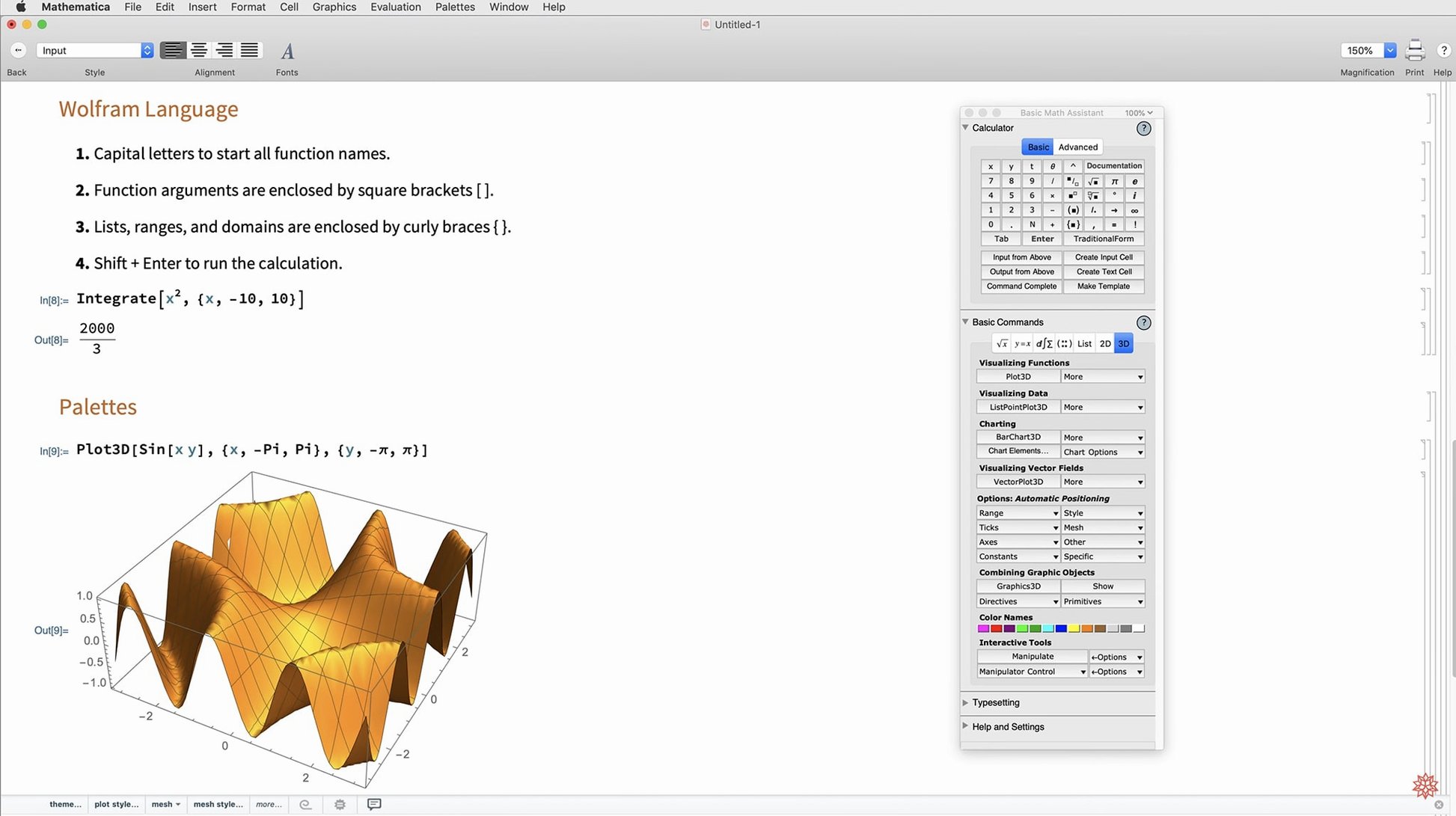
4. Make it visual. Plot your data with ListFitPlot, work with surface plotting functions, or pull in vector-based maps. Mesh processing tools give you more ways to handle 3D geometry.
5. Pull in outside data. Connect to external sources, use the improved Python and R integration, or access Wolfram Cloud through a browser when you're away from your Mac.

You also get tools for building interactive interfaces, geodesic computation, and Markdown export. The interface switches between English, Spanish, Japanese, and a dozen other languages. It's not a light app, but on a supported Mac it settles into being a deep workbench for maths, data, and visualisation.

Dark mode with plot colours that just work

Dark mode isn't a bolt-on here. Notebooks, palettes, and the documentation centre all respect the system setting without odd colour artefacts. The new standard colours for light and dark environments mean your plots look right whichever mode you're in — a small thing that saves you re-styling graphics twice for slides and print.

If you do signal processing, Hilbert transforms now sit alongside the Fourier tools you already use. Lommel functions fill a gap for anyone solving wave problems in cylindrical coordinates. The new matrix decompositions quietly speed up a chunk of linear algebra workflows.

On the everyday scripting side, the faster Python and R integration is the kind of improvement you feel when you call external models and don't wait through a coffee break. ColumnwiseCombine tidies up data-wrangling code that used to need three extra steps. Markdown export is handy for sharing notebooks with colleagues who don't run Mathematica — paste the output straight into a repo README or a lab report.

Free-form input that remembers context

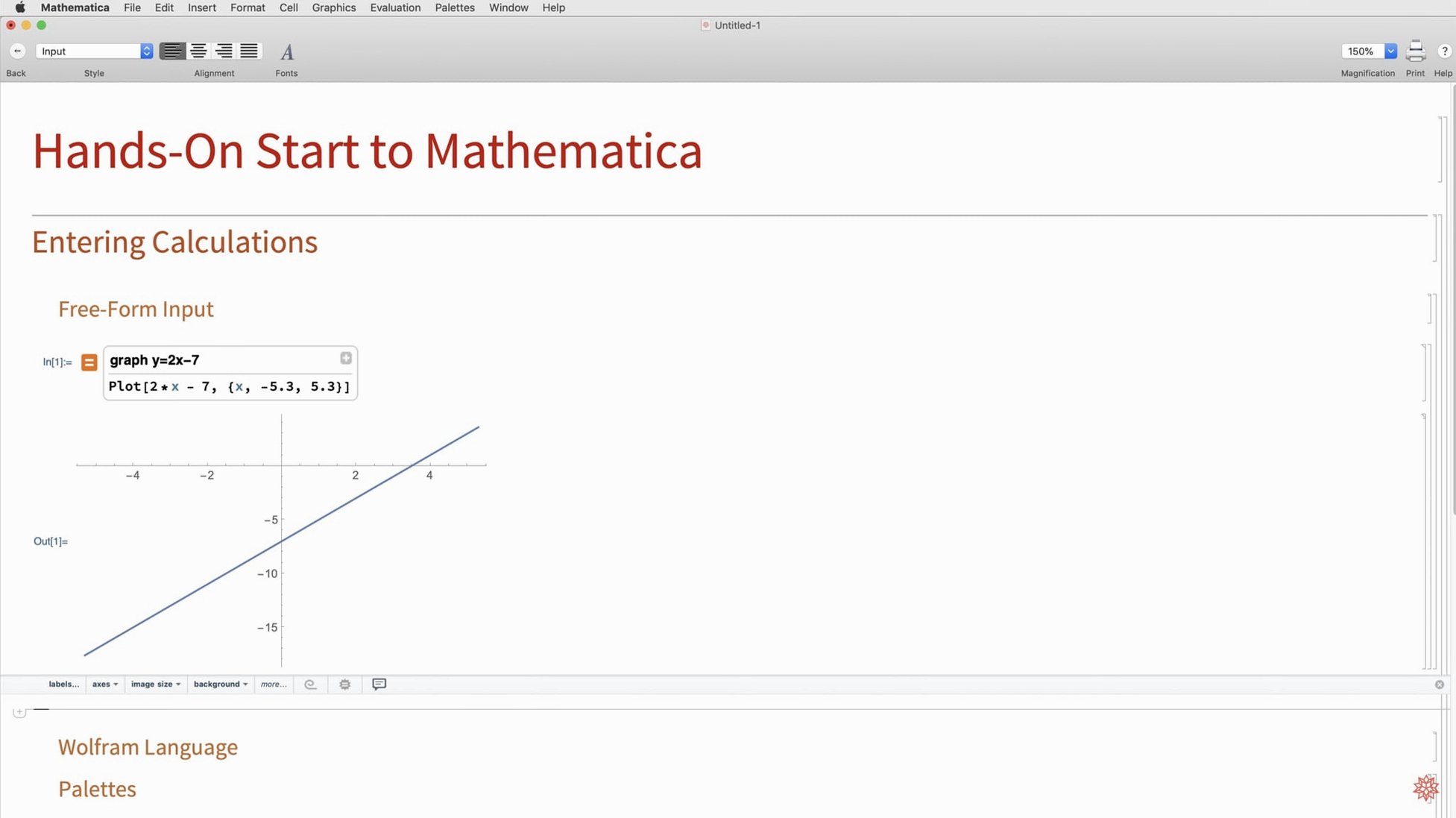
• Free-form input remembers context. Hit equals at the start of a line, type "plot solution to heat equation on a disk," and the Wolfram Language suggestion is usually close. You can fine-tune from there instead of building the whole command from scratch.
• Ctrl-equals for inline Wolfram|Alpha queries. Inside a notebook, you can blend natural language with precise code without opening a browser.
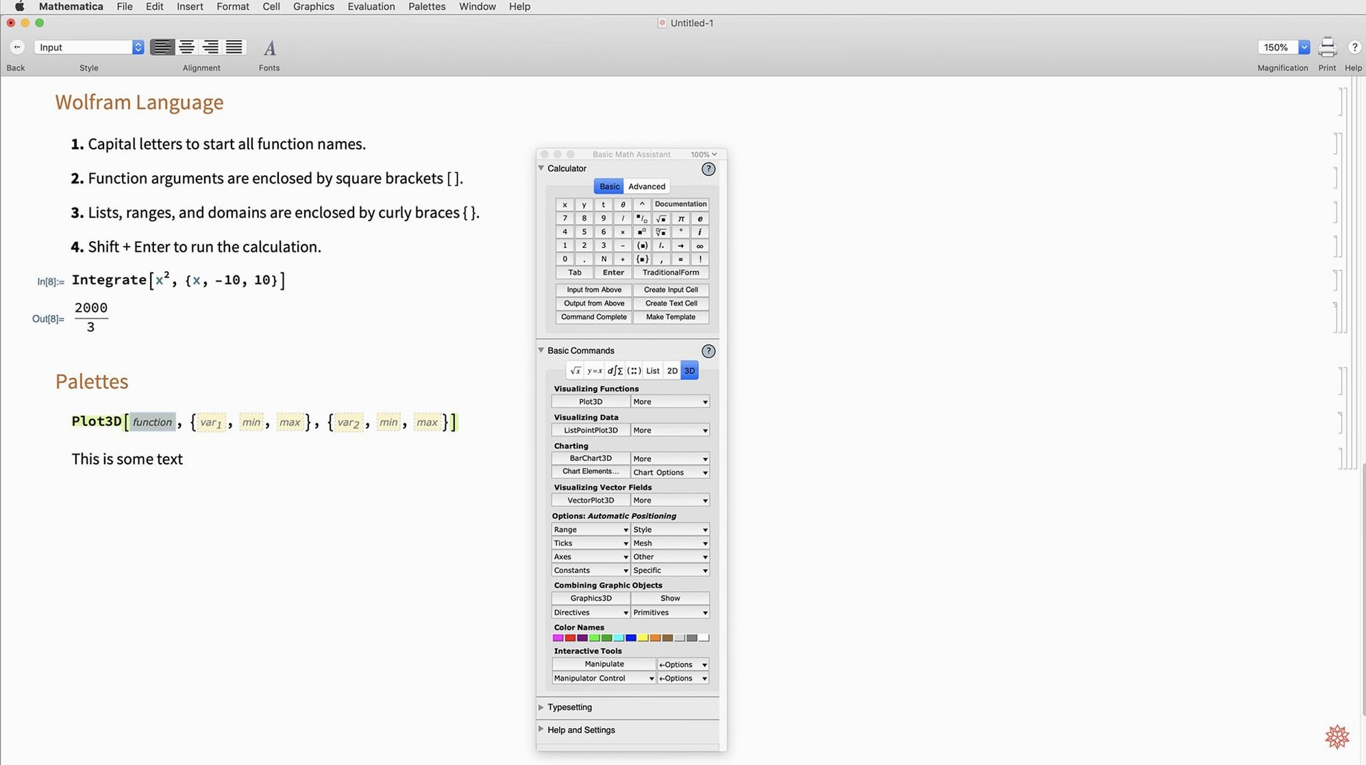
• Palette shortcuts for special characters. The Basic Math Assistant palette gives you clickable integrals, sums, and Greek letters. It's faster than memorising escape sequences when you're still learning.
• Right-click a graphic to copy as vector. Grab a plot as a PDF or SVG, drop it into a Keynote deck, and it stays sharp at any size.
• Autocomplete on function arguments. Start typing ListPlot[ and pause — the tooltip shows argument order and common options. Saves a trip to the documentation.
• Hold Shift when resizing 3D graphics. Lock the aspect ratio so your spheres don't turn into eggs.

Workflow: fitting experimental data to a model

Say you've got a CSV of temperature readings over time from a cooling experiment. You want to fit an exponential decay, visualise the fit, and share the result.

1. Import the data. data = Import["~/Desktop/cooling.csv"]. The notebook auto-detects columns and shows a preview.
2. Plot it raw. ListPlot[data, PlotStyle -> Red] gives you a quick look for outliers or measurement gaps.
3. Define a model. model = a Exp[-k t] + b. The parameters a, k, and b represent amplitude, decay rate, and ambient offset.
4. Run the fit. fit = NonlinearModelFit[data, model, {a, k, b}, t]. Mathematica estimates starting values if you skip them, though good guesses help.
5. Check the parameters. fit["ParameterTable"] shows estimates and confidence intervals so you can judge whether the fit is sensible.
6. Compare fit to data. Show[ListPlot[data], Plot[fit[t], {t, 0, 100}]] overlays the fitted curve. If it's off at the tail, you might need a second exponential term.
7. Export for a report. Right-click the final graphic, choose Save Graphic As, pick PDF. Then Export["fit_results.md", fit["ParameterTable"]] drops a Markdown table into your project folder — ready for the lab write-up.

• Full dark mode support with new standard colours for light and dark environments
• Hilbert transforms and Lommel functions added
• New matrix decompositions
• ListFitPlot, surface plotting functions, vector-based maps, and mesh processing tools
• Geodesic computation and LLMGraph
• Faster Python and R integration
• ColumnwiseCombine, system model validation tools, and Markdown export support

• macOS 12 or later
• Intel or Apple Silicon Mac